

ABSTRACT
We describe a method to extract resonant orbits from N-body simulations, exploiting the fact that they close in frames rotating with a constant pattern speed. Our method is applied to the N-body simulation of the Milky Way by Shen et al. This simulation hosts a massive bar, which drives strong resonances and persistent angular momentum exchange. Resonant orbits are found throughout the disk, both close to the bar and out to the very edges of the disk. Using Fourier spectrograms, we demonstrate that the bar is driving kinematic substructure even in the very outer parts of the disk. We identify two major orbit families in the outskirts of the disk, one of which makes significant contributions to the kinematic landscape, namely, the m:l = 3:−2 family, resonating with the bar. A mechanism is described that produces bimodal distributions of Galactocentric radial velocities at selected azimuths in the outer disk. It occurs as a result of the temporal coherence of particles on the 3:−2 resonant orbits, which causes them to arrive simultaneously at pericenter or apocenter. This resonant clumping, due to the in-phase motion of the particles through their epicycle, leads to both inward and outward moving groups that belong to the same orbital family and consequently produce bimodal radial velocity distributions. This is a possible explanation of the bimodal velocity distributions observed toward the Galactic anticenter by Liu et al. Another consequence is that transient overdensities appear and dissipate (in a symmetric fashion), resulting in a periodic pulsing of the disk’s surface density.
1. INTRODUCTION
Modeling the stellar disk in spiral galaxies often begins with the assumption of axisymmetry. For some purposes, this can be sufficient and is often illuminating and powerful. Real spiral galaxies, however, are not so simple and exhibit a wealth of structure, leading to strong nonaxisymmetries. The Milky Way is host to numerous nonaxisymmetric features, such as spiral arms and the central bar. It has been shown that the majority of bright spirals are host to strong bars (e.g., Eskridge et al. 2000; Marinova & Jogee 2007). N-body simulations of disk galaxies that start out in an axisymmetric configuration often succumb to dynamical instabilities and self-consistently develop bars and spirals (e.g., Sellwood 1981; Debattista et al. 2006; Martinez-Valpuesta et al. 2006). These features can have have a significant effect on the orbital structure in disks, and so it is of great importance to understand these mechanisms and have the right tools at our disposal to analyze models that exhibit these features.
Orbits in nonaxisymmetric systems periodically experience torques introduced by rotating overdensities. Long-lived features allow time for orbits to become resonantly coupled with periodic variations in the torque as the disk evolves. Naturally, this means that the locations of these resonances are strongly linked to the pattern speed of the rotating features and the rotation curve of the disk. The important locations are the resonant radii, such as at the corotation radius (CR) and the location of the Lindblad resonances (LR; see, e.g., Weinberg 1994; Binney & Tremaine 2008). At these locations, the orbits differ drastically from those in axisymmetric models. Deviations from axisymmetry, even in the disk center, therefore cannot be disregarded when trying to explain kinematic structure in the outskirts of the disk. While it has been shown in external galaxies and in simulations that a central bar cannot extend beyond CR (Chirikov 1979; Contopoulos 1980; Sellwood & Wilkinson 1993), it can have observable effects and influence on the dynamics even in the outer parts of the disk.
It is now beyond doubt that the Milky Way is host to a central bar (e.g., Blitz & Spergel 1991; Dwek et al. 1995), yet its characteristic properties are still the subject of debate (e.g., Dehnen 1999; Gerhard & Martinez-Valpuesta 2012). Resonant features induced by the bar have been used to explain the nature of moving groups in the Solar vicinity seen in the Hipparcos and Geneva–Copenhagen Survey data (Dehnen 2000; Minchev et al. 2010). Departures from axisymmetry in the disk have also been suggested as the reason for high values of the vertex deviation in the Solar neighborhood and also low values for the ratio of the principal axes of the velocity-dispersion tensor (Evans & Collett 1993; Dehnen & Binney 1998). Larger-scale surveys, such as the RAVE (RAdial Velocity Experiment; Steinmetz et al. 2006), have recently been used to map the kinematic landscape in the Solar neighborhood (e.g., Siebert et al. 2011; Monari et al. 2014), but the lack of accurate parallaxes and proper motions prohibits an investigation into full six dimensional (6D) phase-space structures over significantly broad areas of the disk. The Sloan Digital Sky Survey (SDSS; Ahn et al. 2012) and, in particular, the Sloan Extension for Galactic Understanding and Exploration (Yanny et al. 2009a) have been of immense value in describing the properties of the Milky Way disk (e.g., Bond et al. 2010; Carollo et al. 2010; Bovy et al. 2012a, 2012b; Smith et al. 2012), in uncovering substructure in the Milky Way’s stellar halo (e.g., Smith et al. 2009; Yanny et al. 2009b; de Jong et al. 2010), and in discovering new Milky Way satellites and characterizing their tidal tails (e.g., Newberg et al. 2009; Belokurov et al. 2010; Koposov et al. 2010). More recently, the (Apache Point Observatory Galactic Evolution Experiment; Eisenstein et al. 2011; Majewski, & SDSS-III/APOGEE Collaboration 2014) infrared (IR) survey has probed the low-latitude regions of the disk, heavily obscured in optical surveys. This large-scale IR survey of the Galactic disk (mostly bright giants and red clump (RC) stars) has allowed us to identify kinematic features associated with the bar (e.g., Nidever et al. 2012; Vásquez et al. 2013), but without accurate distances on the largest scales their interpretation is still the subject of debate (see Li et al. 2014). On smaller scales, but with more accurate distances, the RC sample (Bovy et al. 2014b) has yielded valuable insights into broad streaming motions present in the disk (Bovy et al. 2014a) as well as motions associated with the spiral arms (Kawata et al. 2014) and the Galactic warp (Lopez-Corredoira et al. 2014). Beyond positions and velocities, spectroscopic surveys also permit a view of the chemical landscape of the disk (Randich et al. 2013; Howes et al. 2014; Nidever et al. 2014; Rojas-Arriagada et al. 2014). Obtaining accurate 6D phase-space information along with abundances allows us to probe the evolutionary history of the Milky Way.
Orbits in stellar disks are often described by oscillations in the radial, azimuthal, and vertical directions with respective frequencies, κ, Ω, and ν. Nonaxisymmetric patterns are also characterized by the frequency with which they rotate in the disk, often called the pattern speed,  . A resonance occurs (in the plane of the disk) when there is a commensurability between these frequencies, namely,

or, equivalently,

where l and m are some integer values and TR and  are the epicyclic and the orbital period in the rotating frame, respectively. The component
  is the orbital frequency of the star in the frame rotating with pattern speed
  . In this frame, the orbit completes m radial oscillations for every l azimuthal oscillations. As m and l are integers, the resonant orbit closes in the rotating frame. The integer m also describes the multiplicity of the pattern the closed orbit traces out—the orbit will have m-fold symmetry after l rotations. We note here that, outside of CR, the orbit proceeds in an opposite sense to the pattern with
  . For this reason, we set
  outside CR. With this terminology, the outer Lindblad resonance (OLR) corresponds to the m:l = 2:−1 resonance where
  is necessarily negative, so by keeping
  in this region (beyond CR), Equation (1) is satisfied. At the OLR then, an orbit completes two radial oscillations for every one azimuthal oscillation when viewed in the rotating frame with angular frequency
  .
.
The study of dynamics near resonances has a long history (e.g., Contopoulos 1970; Lynden-Bell & Kalnajs 1972; Lynden-Bell 1973). The classical approach involves perturbations to an axisymmetric model (see Lichtenberg & Lieberman 1983). This line of inquiry gives valuable insights into the dynamics of orbits under small perturbations and is often used in studying linear stability (e.g., Gerhard & Saha 1991; Palmer 1994). The addition of a perturbation series, however, encounters a problem near resonances. This involves the addition of a component with a divisor equal to  , which of course approaches zero at a resonance—the well-known “problem of small divisors” (see, e.g., Arnol’d 1963). This results in a divergence of the solution near a resonance and so does not give a formal answer.
The analysis of resonances in N-body simulations is usually handled by means of a frequency analysis. This requires either measuring the instantaneous frequencies of particles in the simulation or integrating the chosen orbit in a frozen potential that corresponds to the density distribution at some time step in the simulation. Since the emergence of large N-body simulations, this method has become ubiquitous and has proved to be powerful and enlightening. However, the method assumes that angular momentum exchange is minimal and has no significant effect over the course of the orbit. This may lead to errors if angular momentum exchange is both constant and significant. In a potential with a significant perturber, instantaneous frequencies do not give give an accurate representation of the full orbit. This is especially true in the case of resonant orbits in disks with large bars where angular momentum is constantly, and periodically, lost and gained. For this reason, the azimuthal frequency must be calculated over the whole orbit, preferably over one rotation in the rotating frame. Below we outline a simple method to get a robust estimate of Ω (Section 3.1) using only the simulation output.
A Fourier analysis is often employed to extract frequencies and is usually sufficient, but in some cases encounters a problem in the outskirts of the disk where frequencies are low. A slowly changing potential can introduce low-frequency radial modes, and so a lower cutoff is introduced to remove these, but may also remove some orbits in the very outskirts of the disk (Ceverino & Klypin 2007). As we shall see below (Section 4.1), the potentials of N-body simulations rarely have the characteristic of being time-independent. This means that integrating an orbit in a frozen potential will fail to replicate the real N-body trajectory. Also, it is well known that angular momentum exchange between a galactic bar and the halo or a gaseous component to the disk can vary the pattern speed and strength of the bar (Athanassoula 2002, 2003). By choosing a time-independent pattern speed, orbits integrated in frozen potentials lose this characteristic of realistic barred potentials.
Below we introduce a new method for analyzing N-body simulations. Its main aim is to uncover resonant orbits in stellar disks using the fact that, in a rotating frame, the orbit should close and return to a previously occupied region of phase space. We outline the method in Section 2. The method requires little a priori information. It only requires the recalculation of the N-body orbits in many different frames. This approach is then applied to the outskirts of the N-body simulation described by Shen et al. (2010) in Section 3. As a diagnostic tool, we will construct Fourier spectrograms for the disk (Section 3.2) and estimate the radial and azimuthal frequencies (Section 3.1). This is not required to extract a sample of resonant orbits from the simulation, but only aids in their interpretation. We then explore some of the properties of our extracted sample of resonant orbits in Section 4 and discuss our findings in Section 5.
2. PHASE-SPACE DISTANCE METRIC
In a particular rotating frame, a resonant or periodic orbit forms a closed pattern and returns to a previously occupied patch of phase space. Using this, we make a blind search for orbits that return to some arbitrarily selected starting position in phase space. To do this, we recalculate the orbits from our N-body simulation in many different rotating frames. We define a phase-space distance metric, which measures the distance traveled in the rotating frame  . A resonant orbit closes in the rotating frame of its perturber, and so
  for this orbit approaches zero. In practice,
  will not return exactly to zero, so we define some cutoff point, below which the orbit has closed, or nearly so.
N-body simulations give the full orbital history in the inertial frame ( ), which can be recalculated in a rotating frame (
 ). We first define our (arbitrarily chosen) starting position t0 and from there calculate the positions and velocities of particles along their orbits in many rotating frames using a grid of pattern speeds. Since the radial position and velocity are invariant in frames rotating about the z axis, the calculation of the orbit in the rotating frame is trivial. We can write
where  is the frequency of the rotating frame,
  is the duration of the time step (from the N-body simulation,
  Myr), and i is the number of time steps away from the starting point of the calculation. To make a meaningful normalization of phase-space distances, we convert the positions and velocities from polar to Cartesian coordinates (
![$[R^{\prime} ,\phi ^{\prime} ,v_{R}^{\prime },v_{\phi }^{\prime }]\;\to \;[x^{\prime} ,y^{\prime} ,v_{x}^{\prime },v_{y}^{\prime }]$](https://content.cld.iop.org/journals/0004-637X/804/2/80/revision1/apj511178ieqn19.gif) ). For each particle, the distance along each axis of phase space at time step ti is given by
). For each particle, the distance along each axis of phase space at time step ti is given by

Formally, phase space is not a metric space, and so any distance measure is arbitrary and tailored to suit the problem under study. Our general rule of thumb is to first define the expected limits of the orbit in each dimension and normalize accordingly. In this case, we use expectations from simple circular disk orbits. We note that for almost circular orbits,

where  is the guiding radius of the orbit (i.e., the radius of a circular orbit with an equivalent angular momentum). This suggests the following normalization on the spatial component of the phase space,
Since angular momentum exchange is ongoing in the disk, we use the average guiding radius over the course of the orbit,  (note that the guiding radius is evaluated by equating the angular momentum, Lz, of the particle with the angular momentum of a rotation curve derived from azimuthally averaged force calculations). However, the median guiding radius may serve as a better normalization if sampling is far from uniform along the orbit. If an orbit near the center of the disk is sampled with a constant
  , then there will be significantly more points around the apocenter than around the pericenter, skewing the value of
  to higher values. By using either the average or median
  , the spatial component of
  varies between roughly 0 and 1 (see Figure 1). We use a similar method to normalize the kinematic component of the phase-space distance. For almost circular orbits, it is true that

so we can calculate a locally normalized distance using
Here, we have again taken an average of  in the rotating frame over the course of the orbit (a median value may be more appropriate in the inner parts of the disk). As with the spatial component, using
  means that the kinematic component of
  varies between roughly 0 and 1 (see Figure 1). The full phase-space distance is then calculated as

where  varies roughly between 0 and
  .
.

Figure 1. Circular orbits suggest a normalization for our phase-space distance metric. The maximum separation on the (x, y) plane between two circular orbits differing only in orbital phase is twice the guiding radius (left). Using this as our normalization means the spatial component of the phase-space distance varies between 0 and 1. In a similar fashion, the maximum separation of the kinematic component is twice the rotational velocity (right). This normalization forces the kinematic component of the phase space to vary between 0 and 1 as well.
Download figure:
Standard image High-resolution imageThis normalization does introduce separate biases on the spatial and kinematic components. On the spatial plane, the normalization is biased in favor of particles that gain angular momentum over the course of the orbit. A significant gain in angular momentum gives rise to an increase in the guiding radius, thereby lowering the spatial phase-space distance (Dp) measured. In a similar vein, an increase in  gives rise to a lower kinematic phase-space distance. We have checked that this bias is weak for reasonable values of
  and only becomes important when
  is a significant fraction of the guiding radius (
 )—at this point the orbit will have been excluded by any cut made on
  . In any case, resonant orbits experience periodic changes in angular momentum as they complete their orbits, so for closed orbits, the variations cancel.
By measuring the lowest phase-space distance of each particle, we can garner a sample of closed orbits by making a cut below which the orbits are deemed to have closed. In order to diminish the effects of using an arbitrary starting point, which can give spurious results, we use three different starting points (t0). We only accept orbits that have a minimum phase-space distance below our predefined cut using all three starting points. Each starting point is separated by 200 time steps or  Myr, which constitutes a significant fraction of the orbital period. Using this separation means we choose very different orbital phases as our starting points, except of course for those with
  Myr.
Myr.
3. AN APPLICATION TO AN N-BODY SIMULATION
We test this method using the N-body simulation described by Shen et al. (2010). This simulation begins as an axisymmetric disk, which, due to dynamical instabilities (see Hohl 1971; Kalnajs 1978; Sellwood 1981; Toomre 1981), develops a strong bar that persists for ∼4.5 Gyr. The pattern speed of the bar remains relatively stable at ∼38.5 km s−1 kpc−1 for the duration of the simulation because there is no gaseous disk component or live halo to which angular momentum can be deposited. The amplitude of the bar in this case is expected to result in a strong resonant reaction in the disk. The bar also drives recurring transient spirals. This persistent strong bar gives us the opportunity to test the above method in a situation where angular momentum exchange is significant and long-lived, i.e., where a perturbation series and a frequency analysis may have difficulty. The CR of the bar is at  kpc, and the OLR lies in the range
  kpc.
kpc.
The starting configuration of the simulation is an axisymmetric disk embedded in a logarithmic halo with a disk scale length of  kpc and scale height of
  kpc. The disk is comprised of 106 stellar particles with a total mass of
  , whereas the mass of the halo is determined by an asymptotic rotational velocity of
  = 250 km s−1. The simulation was tailored to match the kinematics of the Galactic bulge as observed by BRAVA (Bulge RAdial Velocity Assay; Rich et al. 2007; Howard et al. 2008), and this was used to constrain the angle of the bar with respect to the Galactic center—Solar position line. The final configuration of the system consisted of a bar with a half-length of 4 kpc and an axial ratio of ≈0.5, which is consistent with previous estimates from gas dynamics (Englmaier & Gerhard 1999; Weiner & Sellwood 1999). The final bar angle was ∼20°, again in agreement with previous studies (e.g., Stanek et al. 1997; Bissantz & Gerhard 2002). It has also been recently shown that the simulation is in good agreement with observations of RC stars toward the Galactic center. An X-shaped structure that results from the buckling of the bar (see, e.g., Raha et al. 1991) leads to a bimodal distribution of distances (or magnitudes) for some fields toward the Galactic center (Saito et al. 2011) and is well replicated by both this simulation (Li & Shen 2012) and that of Gardner et al. (2014). In a forthcoming paper (M. Molloy et al. 2015, in preparation), we isolate the resonant orbits that contribute to this feature, describing their kinematic properties.
We apply the method over many epochs during the lifetime of the simulation, finding a good sample of closed orbits at all times after ∼2 Gyr. We focus here on the last gigayear of the simulation (∼4–5 Gyr). As we are particularly interested in orbits resonant with the bar, we limit our search to pattern speeds close to that of the bar ( km s−1 kpc−1). In Figure 2, we plot the density of closed orbits as a function of their average guiding radii and the pattern speed of the rotating frames in which they close. In the upper panel, we impose a cut of
  , and in the lower panel, we impose a cut of
  . By imposing a tighter cut on
  , we extract a “cleaner” sample of resonant orbits. As the cut approaches zero, we converge on the “parent” orbit for each resonance. Looser cuts then encompass orbits that librate about the parent orbit. In Table 1, we list the number of resonant orbits extracted for each cut. There are many more resonant orbits within CR. The choice of cut therefore depends on the region in question.
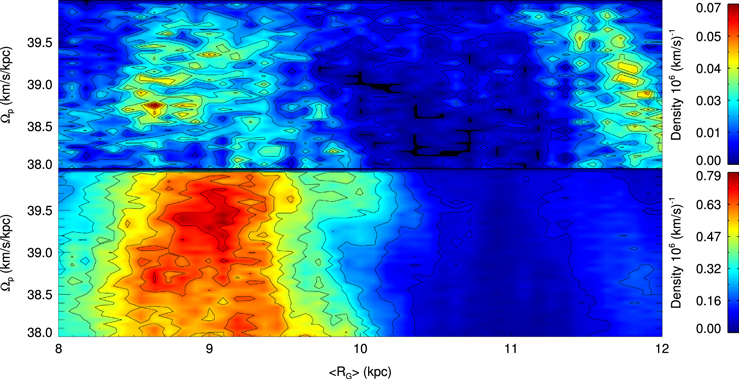
Figure 2. Density of closed orbits as a function of their average guiding radius and the pattern speed for which they close. We study various rotating frames with frequencies in the range  km s−1 kpc−1 using a grid of
  km s−1 kpc−1. The top panel indicates our selection when the minimum phase space achieved is less than
  , and the bottom panel is when
  . Most of the closed orbits have
  kpc with a smaller contribution from orbits with
Download figure:
Standard image High-resolution imageTable 1.
By Imposing Stricter Cuts on the Minimum Phase-space Distance  , We Extract Samples of Cleaner, More Strictly Closed, Orbits
Cut ( Cut) Cut) |
Total |
 kpc kpc |
 kpc kpc |
|---|---|---|---|
| No Cut | 977,357 | 680,005 | 297,352 |
| 0.1 | 529,015 | 424,097 | 104,918 |
| 0.08 | 425,788 | 355,854 | 69,934 |
| 0.06 | 297,186 | 255,247 | 41,939 |
| 0.04 | 141,061 | 121,747 | 19,314 |
| 0.025 | 40,744 | 35,478 | 5266 |
Download table as: ASCIITypeset image
Here, we extract a sample of closed orbits whose distribution of guiding radii peaks at ∼9.0 kpc and closes in a rotating frame close to the pattern speed of the bar (∼38.5 km s−1 kpc−1). In order to measure the pattern speed, we compute the numerical derivative of the phase angle of the m = 2 Fourier component within CR over a number of time steps. The pattern speed of the bar remains constant at ≈38.5 km s−1 kpc−1 for most of the duration of the simulation (see also Section 3.2).
A source of ambiguity remains, however. An orbit can close in many frames. Specifically, an orbit with epicyclic (κ) and orbital frequency (Ω) closes in a frame  for which
Here, the subscript m:l indicates that the orbit closes with m radial oscillations for every l azimuthal oscillations in that frame. When we reproduce Figure 2 over a much wider range of pattern speeds ( km s−1 kpc−1), we see multiple overdensities corresponding to this degeneracy. Therefore, while we have limited our search for resonant orbits associated with the bar, we may also be extracting orbits that are driven by slower or faster moving patterns and which also happen to close in a frame close to that of the bar’s. To clarify the matter, we measure the orbital and epicyclic frequencies for our sample of closed orbits. Using this information, we determine the pattern speeds of the rotating frames in which our orbits will close for various families of orbits (e.g., m:l = 1:-1, 1:-2, etc.).
3.1. Measuring Frequencies
It is difficult to estimate reliably the orbital frequencies of stars in disks in which angular momentum exchange is persistent and significant. Taking instantaneous measurements of the azimuthal frequency Ω introduces an error because the angular momentum at one point in the orbit may be, sometimes significantly, different from that at another point. For this reason, it is better to estimate the frequency over the course of a full orbit. This is especially true for resonant orbits—the periodic loss and gain of angular momentum is averaged out over some integer number of azimuthal oscillations in the rotating frame.
Our method makes use of the fact that an orbit plotted in a rotating frame with the same frequency as the orbital frequency of its guiding center will trace out an ellipse (its epicycle) that appears stationary. In this frame, the epicycle does not precess around the center of the disk and explores only a limited range in ϕ. In each rotating frame, the orbit has a minimum and maximum azimuth ( and
and  ). The range in ϕ traversed by the orbit is
  . The method minimizes
  by scanning various rotating frames with higher and higher resolution until the variation between adjacent frames reaches some predefined limit. For well-behaved orbits, this converges to the true orbital frequency of the guiding radius. The epicyclic frequency is easily extracted from the period of the radial oscillation.
3.2. Fourier Components
Discerning which of the nonaxisymmetric features of the disk (e.g., the central bar or spiral arms) resonate with our closed orbits requires an analysis of the wave patterns that propagate through the disk. For this, we decompose the disk into its Fourier components. We follow the procedure outlined by Quillen et al. (2011) to construct our spectrograms. For equally spaced radial bins at each time step, we measure
where we sum over all j particles in each radial bin. We then numerically integrate over the complex function

where we sample over the frequency domain  km s−1 kpc−1. We also use a Hanning window function h(t) that spans the time window T1 to T2. We construct spectrograms using the m = 1, 2, 3, and 4 Fourier components for five different time windows with
  Gyr (1000 time steps) from ∼2 to ∼5 Gyr (i.e., 2
  3 Gyr, 2.5
  3.5 Gyr, 3
  4 Gyr, etc.). The spectrograms are sampled every 9.6 Myr (10 time steps) so that we can uncover transient features (such as spiral arms) that require a high temporal resolution.
The m = 1 and 3 spectrograms exhibit patterns many orders of magnitude weaker than the m = 2 patterns, while the m = 4 spectrograms show only the first harmonic of the m = 2 patterns. We give only the m = 2 spectrograms in Figure 3 with the vertical axis indicating the pattern speed and the horizontal axis the radial extent of the features. The color shows the strength of the feature (in arbitrary units and on a log scale). We show CR as the black line and also the 2:±1 LR as blue lines. The m:l LR are derived from the rotation curve calculated using force measurements around the disk. This gives  , the azimuthal frequency of circular orbits at R. Using a numerical differentiation of
  , we derive
  from
from
The m:l Lindblad Resonance/Radius (LR) is then (where, as before,  for R exceeding the CR)


Figure 3. m = 2 Fourier spectrograms spanning  Gyr. From left to right, the spectrograms probe the time range from 2
  3 Gyr, 2.5
  3.5 Gyr, 3
  4 Gyr, 3.5
  4.5 Gyr, and 4
  5 Gyr. In constructing our spectra, we sample the disk every ∼10 Myr and use a Hanning window function to bracket T1 to T2 (Equation (12)). The color bar denotes a log scale in arbitrary units. We also indicate CR with the black line and the 2: ±1 LR with the blue lines (Equations (13) and (14)). The most prominent pattern is that of the bar, which is rotating with a pattern speed of ∼38.5 km s−1 kpc−1. It extends from the center of the disk out to its CR at ∼4.5 kpc. A two-armed spiral emanates from the ends of the bar, which also overlaps with a slower spiral feature at ∼25 km s−1 kpc−1. We also see the emergence of a transient feature at ∼15 km s−1 kpc−1.
Download figure:
Standard image High-resolution imageThe spectrograms of the m = 2 Fourier components indicate the radial extent and the rotational frequency of two-armed structures, like a bar or spiral arms, in the disk. The most prominent feature is the bar pattern, which extends from the center of the disk out to its CR, rotating at ∼40 km s−1 kpc−1. A weaker feature extends from the end of the bar in all m = 2 spectrograms and reaches as far as the 2:-1 LR. The orbits that make up the structure of the bar are prohibited from extending beyond corotation (see Chirikov 1979; Contopoulos 1980), so this feature is likely due to spirals emanating from the ends of the bar. We see another two-armed structure that also extends from the end of the bar, but rotates with a lower frequency (∼22 km s−1 kpc−1). At later times, a further spiral is seen at a still lower frequency (∼15 km s−1 kpc−1). This spiral has its ILR at the same radius as the bar’s CR, which may indicate the presence of mode-coupling (Tagger et al. 1987; Minchev et al. 2012). The bar is extremely stable in this simulation and only slows down very slightly over the last 4 Gyr. The spectrograms indicate clearly the presence of multiple patterns in the disk, which contribute to the ambiguity about the forcing resonant perturber.
3.3. Diagnostic
We now calculate the pattern speeds in which orbits close for various values of m and l ( , Equation (10)). Using this along with our Fourier spectrograms, we can decipher the most likely resonant origin for our sample of closed orbits. We make two assumptions in the following analysis.
- 1.Resonant orbits occur due to nonaxisymmetric patterns inside the guiding radii of the orbits.
- 2.Resonant orbits occur roughly at the location of a LR (see Binney & Tremaine 2008, Section 3.3.3).
By plotting our  distributions over our m = 2 spectrograms, we look for the coincidence of the distributions with nonaxisymmetric features in the disk, satisfying our assumptions above. We neglect the m = 1, 3, and 4 spectrograms because the amplitudes of those patterns are dwarfed by the m = 2 components.
Figure 4 shows the m = 2 spectrograms for the final gigayear of the simulation (the rightmost plot in Figure 3). The spectrograms are identical in each plot. We have overlain the distributions of  for the 1:-1, 2:-1, 3:-1, and 3:-2 (first, second, third, and fourth plots, respectively) orbit families as the blue dots. The blue dots in each of the plots mark the same particles. We have chosen only the particles that have
  , namely, the “cleanest” or “most closed” orbits. Their different position in each plot represents the different frames in which they close as different types of orbits. We identify two separate groups of closed orbits with significantly different distributions in
  —one lies inside 11 kpc, whereas the other lies outside. For both groups, we have plotted the median frequency in each distribution (given by the horizontal line).
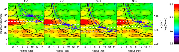
Figure 4. m = 2 component spectrogram covering the time window 4  5 Gyr, i.e., the rightmost plot in Figure 3. Each plot shows the same spectrogram, with the CR indicated as the black line. We indicate the m:l LR as the blue and red lines—the 1:-1 LR in the first plot, the 2:-1 LR in the second plot, and so on. The red line uses the epicyclic approximation (i.e., κ is derived from the rotation curve,
  ), whereas the blue lines use the median κ from samples of orbits. Specifically, the outer blue line uses the median κ from the particles in the range
  kpc, whereas the inner blue line uses the median κ from particles with
  kpc. In each plot, we overlay the distributions of
  (Equation (10)) for particles with
  as the blue points—they represent the same particles, the only difference being the frequency of the rotating frames in which they close as 1:-1 (first), 2:-1 (second), 3:-1 (third), and 3:-2 (fourth) orbits. The median frequency of each
  distribution is plotted as the horizontal dashed line. Two separate groups appear at distinct frequencies. The larger group (with higher frequencies) is coincident with the 3:-2 LR and is in good agreement with the pattern speed of the bar as a family of 3:-2 orbits. The lower-frequency group could be resonating in a 1:-1 fashion with the strong bar pattern or in a 3:-1 fashion with a weaker pattern at ∼22 km s−1 kpc−1.
Download figure:
Standard image High-resolution imageWe also overplot the LR curves (blue/red) along with the CR curve (black) for the disk (the rotation curve is almost constant over the duration of the simulation, so we use the curves as they are at the end of the simulation). The 1:-1, 2:-1, 3:-1, and 3:-2 LR are shown in the first, second, third, and fourth plots, respectively. For the LR curves, we have used two different approaches corresponding to the blue and red lines. The red LR curves use  , which is evaluated from the epicyclic approximation using numerical differentiation (Equation (13)). The blue LR uses the median κ from the sample of resonant orbits along with
  . For the outer (inner) LR, we use the median κ of the orbits inside (outside) 11 kpc. (Note that these curves are only valid over the radius spanned by the blue points). Also, the particles generally rotate slower than indicated by the rotation curve, meaning that
  is an overestimate of the true Ω. This means that at a given radius the frequency of the LR is also slightly overestimated.
To begin with, we focus solely on the group with  between 6 and 11 kpc. We look for coincidence of the blue points (the distributions of
  ) with both a strong pattern (the red/yellow peaks in the spectrogram) and the location of a LR (the red/blue lines). We can see that the distributions of
  (the blue points) only satisfy our assumptions above for the m:l = 3:-2 orbit family (fourth plot). In this case, the guiding radii of the orbits are coincident with the 3:-2 LR and have almost the same pattern speed as the bar (∼40 km s−1 kpc−1). This is good evidence that the group of periodic orbits inside 11 kpc are resonating in a 3:-2 fashion with the bar. The distributions of
  are not coincident with any strong pattern as 1:-1, 2:-1, or 3:-1 orbits.
Similarly, for the group of orbits that lie outside 11 kpc, we see that they satisfy our assumptions in the m = 2 spectrogram for the 1:-1 orbit family. First, as a family of 1:-1 orbits, they close in a rotating frame with almost the same pattern speed as the bar. Second, their location on the spectrogram coincides with the 1:-1 LR. There is also some agreement for the 3:-1 orbit family—a small feature lies inside the distribution with  km s−1 kpc−1. However, since the bar is much stronger than the pattern at ∼22 km s−1 kpc−1, it is likely that these orbits are resonating in a 1:-1 fashion with the bar. Only a handful of particles inhabit this resonance (∼1750 for
  and ∼2300 for
  ), and they make no significant contribution to kinematic structures in the disk (even though they make up ∼20% of all particles with
  kpc for both cuts), so we do not consider them further. The 3:-2 orbits make up only ∼1% of all particles with
  kpc for
  but increase to over 30% for
  .
.
We remark that the measured frequencies (Ω and κ) are estimates of the true frequencies. They do, however, serve well as a diagnostic and remove any ambiguity regarding the forcing resonant perturber. By estimating the frames ( ) in which our sample of resonant orbits close as different orbit types, we can ignore families for which there are no patterns with commensurate frequencies. For example, we see that for the 2:-1 orbit family (second plot), there are no patterns that could force this type of resonance, and so we disregard it. The best agreement lies with the bar pattern being the forcing perturber for the 3:-2 and 1:-1 orbit families.
4. RESONANT ORBIT DYNAMICS
Our sample of resonant orbits represents kinematic substructure in the disk that is not present in an axisymmetric potential. The choice of a cut on the minimum phase-space distance may seem arbitrary and does introduce uncertainty on the fraction of particles on resonant orbits. However, it does demonstrate the types of resonances that are populated and can persist for a significant duration in disks with a strong central bar. By extracting a sample of resonant orbits from N-body simulations, we can also look more closely at their behavior as the disk evolves. Here, we concentrate on resonances beyond CR, but this method works just as well for the bar orbits.
4.1. Resonant Clumping
Our 3:-2 orbits behave in a highly coordinated fashion. They are not distributed evenly around the orbit, but instead exist in multiple populations that vary in their epicycle and azimuthal phase. In the following, we describe populations that are in-phase in epicycle as groups. Within these groups are populations with the same azimuthal phase which we call subgroups. With this nomenclature, the groups all reach their pericenters/apocenters at the same time, whereas the subgroups have their pericenters/apocenters at different azimuths. Figure 5 shows the two possible orientations of the 3:-2 orbit—each orientation has one pericenter at either end of the bar that is aligned with the x axis, and the orbits move in a clockwise fashion (in the inertial frame the disk rotates in an anticlockwise fashion). Since we have defined l to be negative for orbits beyond CR, Equation (10) means that  is always larger than Ω, the orbital frequency in the inertial frame (at least for orbits with
  ). The orbital frequency in the rotating frame,
  , is then necessarily negative, i.e.,

so that in the rotating frame the orbit moves in an opposite sense to the inertial frame. It is useful here to define a chirality, or handedness, for each orientation. Those orbits that have one of their pericenters on the negative x axis are left-handed (i.e., on the left end of the bar—the blue orbit), whereas those with one of their pericenters on the positive x axis are right-handed (the red orbit).

Figure 5. Possible orientations of the 3:-2 orbit, which has two-fold symmetry with respect to the bar aligned with the x axis. We define a chirality so the the orientation with a pericenter on the negative x axis is left-handed (blue) and that with a pericenter on the positive x axis is right-handed (red). The orientations of the 3:-2 orbit family allow six possible pericenters (and apocenters). When we overplot the two orientations, we can identify locations (with respect to the bar) at which there are both inward and outward moving groups (indicated by the black ovals). In the inertial frame, the bar and particles rotate in an anticlockwise fashion. In the rotating frame with  , the bar remains aligned with the x axis, and the particles move in a clockwise fashion. The locations occur on the trailing side of the bar at longitudes similar to the Solar position.
Download figure:
Standard image High-resolution imageIf the particles populating these types of orbits are distributed uniformly in azimuth, then we should see bimodal vR distributions at a number of discrete angles with respect to the bar. This is not the case, however. When we measure the times at which the particles reach their pericenters, we see that they are arranged in such a way as to reach their pericenters at almost the same time. Figure 6 shows the distribution of times at which our closed 3:-2 orbits pass through their pericenters. This is clear evidence that the particles are not uniformly distributed, and so we expect a resonant clumping of the particles in azimuth as all of the particles coherently reach their pericenters. It is also clear that the 3:-2 resonant orbits are split into two distinct groups whose epicycles are out of phase by π. The median κ for the 3:-2 orbits is  km s−1 kpc−1, which equates to an epicyclic period of
  Myr. Figure 6 shows that, as one group of 3:-2 orbits reaches pericenter, the other reaches apocenter. The groups then pass each other as they each complete their epicyclic motion—i.e., they comprise an outward moving group and an inward moving group. This coordinated movement gives rise to transient overdensities at pericenter and apocenter and to bimodal distributions in vR.
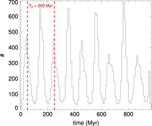
Figure 6. Distribution of times at which our closed orbits reach their pericenters (over the last 0.96 Gyr). Note that the orbits mostly conspire to reach their pericenters at roughly the same time. This is the phenomenon of resonant clumping in the phase angle  (where
  ). We indicate the epicyclic period, TR, for our sample of 3:-2 closed orbits as the vertical red lines. Peaks occur on a timescale of one half of TR, which means our closed orbits are made up of two groups whose epicyclic motion is out of phase by π.
Download figure:
Standard image High-resolution imageWe have checked that this phenomenon is not some artifact introduced by our use of the phase-space distance method. By estimating Ω and κ for a random sample of 10% of the simulation particles, we extract an independent sample of 3:-2 periodic orbits. This sample also exhibits clumping on timescales consistent with the epicyclic period and confirms that no bias toward certain epicyclic phases is introduced.
Each group is host to a number of subgroups. When a group reaches pericenter, its constituent subgroups populate overdensities, which occur at different azimuths. The preferred azimuths have distinct locations with respect to the bar—the allowed locations correspond to the six pericenters shown in Figure 5 (three red and three blue). It is not necessary for all six locations to be populated, but in order to avoid lopsidedness, if one is populated, then another on the opposite side must also be populated with a similar number of particles. We follow these coherent motions by plotting the surface density of the 3:-2 resonant orbits at times when a pericenter/apocenter is reached (Figure 7). The surface density maps in each column are identical and are plotted when a peak occurs in the distribution of pericenter times in Figure 6. In each map, the bar is aligned with the x axis. In the first column, we see four overdensities that lie along the x axis—two inner and two outer, marked by the red circles in each row. The inner overdensities (with  kpc) correspond to a single group, labeled group A. Each (inner) overdensity then corresponds to a subgroup of group A. These subgroups are in-phase with respect to their epicycles but are exactly π out of phase in their azimuthal motion. Similarly, the outer overdensities on the x axis (with
  kpc) constitute group B, whose epicycles are out of phase by π compared to group A. As with group A, group B is host to subgroups—those subgroups on the x axis are also π out of phase in azimuth. So, to reiterate, two overdensities in group A are denoted by the red circles in rows one and three, with both rows indicating separate subgroups. Rows two and four indicate two of the overdensities from group B with, again, each row indicating separate subgroups. For each separate subgroup, we choose a particle and follow its trajectory through successive apocenters/pericenters. In all cases, the bar is aligned with the x axis, and the orbits progress in a clockwise direction.
Figure 7. Surface density maps of the sample of 3:-2 closed orbits only. The long axis of the bar is aligned with the x axis. In each column, the surface density maps are identical. Successive columns show the surface density each time a pericenter or apocenter is reached, as inferred from the histogram in Figure 6 (every ∼100 Myr =  /2). In the first column, we identify four overdensities that lie on the x axis—each row indicates a different one with the red circle. We define a group as those particles whose epicyclic motion is in-phase, i.e., they reach their pericenters or apocenters at the same time. The overdensities indicated on rows one and three represent particles from group A because they both are at pericenter. Overdensities from group B are indicated on rows two and four—they both reside at apocenter. We follow the orbital trajectory of a particle from each overdensity in the frame rotating with the bar—the orbits all move in a clockwise direction. Group A orbits move from pericenter to apocenter, whereas Group B orbits do the converse. Each of the orbits traces out a 3:-2 orbit pattern, with the top two rows exhibiting a left-handedness (the blue orbit from Figure 5) and the bottom two rows exhibiting a right-handedness (the red orbit from Figure 5). We include an animation of the evolution of the 3:-2 orbits as supplementary online material.
(An animation of this figure is available.)
Download figure:
Video Standard image High-resolution imageIn the second column, the particles from group A have moved from pericenter to apocenter, and vice versa for group B. At some intermediate point, the particles from each group have passed each other, with group A having positive vR and group B having negative vR. This passage generates a bimodal distribution of vR in the regions of space where the two groups pass each other. As we move to the third column, group A has returned to pericenter, while group B has moved again to apocenter. Each successive column indicates a pericenter or apocenter until the final column, where the 3:-2 orbit has been completed. In terms of chirality, each group is host to both left- and right-handed 3:-2 orbits (the top two rows are left-handed, and the bottom two are right-handed). Note also that for this simulation, each group is host to four out the six possible subgroups. This is evidenced by the absence of an overdensity at the end of the bar in every third snapshot. If all six subgroups were populated, then each time a pericenter is reached, an overdensity would appear at the ends of the bar.
The evolution of these distinct orbital groups and subgroups leads to a “pulsing” of the density distribution in the disk, with stars periodically and coherently moving inward and outward. These transient overdensities contribute to the time-dependent, but periodic, nature of the galactic potential. The presence of these two populations contributes to stabilizing what seems to be an inherently lopsided configuration. This mechanism of coherence among the resonant orbits suggests that strong kinematic features can be generated as inward and outward moving groups encounter each other.
4.2. Kinematic Signatures
This bimodal distribution of vR constitutes a potentially observable feature from the Solar position. At some point, overdensities appear in line with the long axis of the bar on one side of the disk, one due to an accumulation at pericenter and one due to an accumulation at apocenter (one from groups A and B; e.g., rows 1 and 2, Figure 7). As they both progress to the extremes of their respective epicycles, the bar moves ahead in azimuth. This means that they pass each other on the trailing side of the bar, generating a bimodal distribution in vR. This bimodal distribution appears at distinct azimuths—specifically, between the allowed locations for the pericenters and apocenters (see Figure 5).
The angle of the bar with respect to the line joining the Sun and Galactic Center is poorly constrained. It is estimated to be in the region of 10°–40°(e.g., Stanek et al. 1997; Freudenreich 1998; Robin et al. 2012; Cao et al. 2013; Wang et al. 2013). For an angle of ∼20° on the trailing side of the bar, there is a bifurcation in the radial velocities between 10 and 11 kpc. We indicate these regions with the black ovals in Figure 5. We can simulate a field of view toward the anticenter and measure the distribution of vR as a function of galactocentric distance  . By doing this for only the resonant orbits, we can see how the bimodal nature of the vR distribution emerges (Figure 8). If we rotate the disk so that the bar is at an angle of 20° with respect to the x axis and select only particles that have
  kpc and
  kpc, a bimodal distribution of vR is present between 10 and 11 kpc. This feature is still significant when we consider all (i.e., resonant and nonresonant) particles (left, Figure 8).
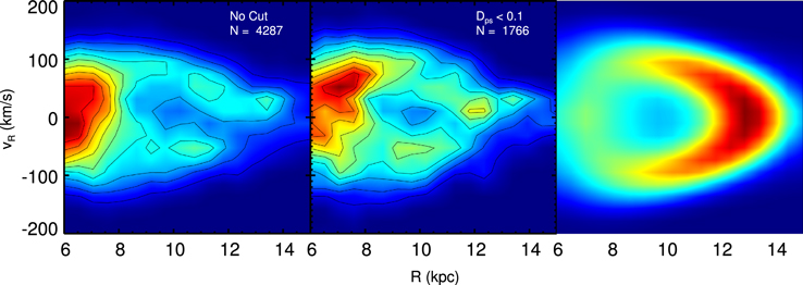
Figure 8. Distribution of vR as a function of R for a pencil beam toward the anticenter at 4.8 Gyr. The number of particles N is also indicated. The disk is rotated so that the bar is at an angle of 20° with respect to the x axis. Particles for which  kpc and
  kpc make up the distributions. On the left, we show the distribution for all particles. A strong kinematic feature is present, namely, the bimodal distribution of vR between 10 and 12 kpc. The middle plot shows the distribution generated by only the resonant orbits using a cut on the phase-space distance of
  . The right plot shows the time-averaged imprint of the resonant orbits in R – vR space. The density in this plot is a measure of the time spent at each location, meaning that the persistence of kinematic features scales with the radius at which they occur.
Download figure:
Standard image High-resolution imageThis result is in good qualitative agreement with the recent observations of Liu et al. (2012) who, for a sample of RC stars in a pencil beam toward the Galactic anticenter, find a bimodal distribution of heliocentric (line of sight) radial velocities,  . The distribution of radial velocities has two significant peaks falling in the range
  kpc at
  km s−1 and
  km s−1. Since the field is directed toward the anticenter, the line of sight velocities
  serve as a good proxy for the galactocentric radial velocities, vR. For the anticenter, we have

By correcting for the radial Solar motion, which has an inward motion of  km s−1, the distribution becomes symmetric about
  = 0 km s−1 with peaks at roughly ±15 km s−1.
Liu et al. (2012) suggest that this feature is due to a resonant interaction with the Milky Way’s bar because their locations are consistent with the position of the OLR. The bimodal distribution in our simulation occurs outside the bar’s OLR (∼8.5 kpc). Since our disk is kinematically hot ( km s−1 at R = 9 kpc), the difference between the two peaks in the velocity distribution is larger than the observations. We have, however, provided a possible mechanism for such a feature to arise. If the resonance is populated in a hot disk, then it is likely to be still more important in a colder disk. In hotter disks, the larger velocity dispersions of stars mean they are less likely to become and remain trapped in narrow resonances.
Finally, in the right plot of Figure 8, we show the time-averaged imprint of the 3:-2 orbits in  space. The vertical and horizontal extent of the distribution is a measure of the epicycle energy associated with the orbits, and the density can be thought of as a measure of the time spent by the particles in these regions. The particles spend little time at pericenter, with the majority of the orbit spent at large R. Kinematic structures due to the resonant orbits are therefore more persistent if they occur in the outskirts of the disk.
5. DISCUSSION
To our knowledge, there has been little investigation of resonant orbits in the outskirts of barred N-body disks. Resonant clumping therefore seems to be a previously unknown phenomenon. For this reason, we discuss the mechanism that causes the periodic orbits to become clumped in phase angle ( ) and to remain so for long periods in the evolution in the disk. In the following, we address two questions: (1) How do the periodic orbits become clumped in the first place? and (2) Why do they remain clumped when phase mixing should work to undo the clumping?
5.1. Resonant Clumping: Origins
To investigate the first point, we apply the phase-space distance method described in Section 2 over many epochs during the evolution of the disk. Specifically, we use eight ∼1 Gyr time segments, from ∼0.5 to ∼1.5 Gyr, ∼1.0 to ∼2.0 Gyr, and ∼1.5 to ∼2.5 Gyr, all the way up to ∼4.0 to ∼5.0 Gyr, which was the segment we analyzed in the previous sections of the paper. We avoid using data from the epoch of bar formation (0–500 Myr) because angular momentum is violently redistributed throughout the disk. The resulting variations in the guiding radii and rotational speeds make the normalizations on the phase-space distance unreliable. In any case, we are able to extract resonant orbits from all eight segments. The number of resonant orbits increases with time and begins to flatten out after segment five (i.e., from ∼2.5 Gyr onward). We also find, by analyzing the azimuthal and radial frequencies, that the 3:-2 orbit family is the dominant family, even from early on.
For our current purposes, we are interested in particles that are captured into resonance early on and that remain in resonance for a long time. To select such a long-lived resonant sample, we take particles found during segment two (∼1 to ∼2 Gyr) and compare them to the particles found during segment eight (∼4 to ∼5 Gyr). Particles that are common to both samples have remained in resonance for at least ∼4 Gyr.
Due to the changes in angular momentum (and the corresponding changes in  and Ω), especially during the formation of the bar, a reliable measure of the phase angle
  (i.e., the clumped angle) is unavailable to us. For this reason, we continue to use the times at which the particles reach pericenter as an indicator of whether clumping in the phase angle is present or not. While this is a robust indication of the presence of clumping, we are unable to say if the particles become clumped in the time period between apocenter and pericenter. In Figure 9 (top panel), we show the distribution of pericenter times for the 3:-2 particles extracted from segment two (∼1 Gyr to ∼2 Gyr; black) and the 3:-2 particles that are common to segment two and segment eight (the long-lived resonant particles; blue). The distributions are shown from t = 0 Gyr to
  Gyr and indicate that the particles become clumped during the formation of the bar (between 200 and 500 Myr).
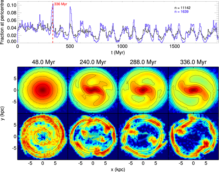
Figure 9. Clumping occurs early on in the evolution of the disk. In the top panel, we show the distribution of pericenter times for particles extracted from segment two (black) and particles common to segments two and eight (blue). The surface density of the disk during the formation of the bar is shown in the top row of the bottom panel (contours of equal surface density). The resonant particles exhibit overdensities at the Lagrange points at either end of the bar (contours of equal effective potential, as shown in the final row).
Download figure:
Standard image High-resolution imageIn the bottom panel of Figure 9, we show the surface density of all particles in the disk (top row) during the formation of the bar with contours of equal density. The bar in this case forms very quickly (within 300 Myr), and its arrival induces strong spiral structures. We also show the surface density for our sample of 3:-2 particles from segment two in the bottom rows, this time with contours of equal effective potential. The outline of the resonant orbits exhibits a striking resemblance to the large ringed-shaped features seen in external barred galaxies (the so-called “R” rings of Buta 1986). It is also clear that overdensities appear close to the Lagrange points at either end of the bar (i.e., L1 and L2). Given that (1) the periodic orbits are clumped in  as the bar is forming, (2) the bar induces strong spirals, (3) the resonant particles appear to follow the pattern of rings in barred galaxies, and (4) overdensities appear close to the Lagrange points, we naturally suspect that the clumping is related to the mechanism that generates these type of structures—namely, passage through the unstable Lagrange points and their associated manifolds.
The mechanics of bar-induced spirals and large-scale rings in barred galaxies has been studied in detail (for comparison, see Gómez et al. 2004; Romero-Gómez et al. 2006, 2007; Athanassoula et al. 2009a, 2009b). The first main point relevant to our work is that L1 (and L2) are host to the Lyapunov orbits (roughly elliptical orbits that corotate with  ). Because the region is unstable, the periodic Lyapunov orbits cannot indefinitely trap other regular orbits. Orbits that visit this region tend to leave it on a timescale proportional to their energy, i.e., lower-energy orbits escape the region faster than orbits with a higher energy. The second main point is that the trajectories through which the orbits (which may have been temporarily trapped) can leave this region are determined by the unstable manifolds—whereas the stable manifolds describe the trajectories through which orbits approach this region. As an example, we plot some orbits that follow these manifolds in Figure 10. Note that not all of the resonant orbits approach the Lagrange points. From the total sample of resonant particles, we estimate that about 75% approach the Lagrange points. For these, the average radius at t = 0 Myr is
  kpc, with
  kpc. In the left (right) panel, we show orbits that come from the inner (outer) parts of the disk. At
  Myr, the majority of particles have
  kpc, indicating passage along the inner stable manifold (i.e., along the bar). The green crosses indicate the positions corresponding to the time at which the surface density and equipotential contours are plotted. The orbits can be compared with those shown in Figure 4 of Athanassoula (2012).
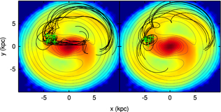
Figure 10. Surface density of all particles at ∼200 Myr with contours of equal effective potential  . Left panel: trajectories of periodic orbits that approach L1 from the bar. Right panel: trajectories of periodic orbits that approach from the outer disk. The orbits are plotted from ∼100 to 450 Myr. The green crosses indicate the positions at ∼200 Myr. The particles move in a clockwise direction (in the frame corotating with the bar).
Download figure:
Standard image High-resolution imageThe third, and possibly most important, point in this context is that the L1 and L2 points can be stabilized by concentrations of matter (see Section 5 of Athanassoula et al. 2009b). This generates a local minimum in the potential, a stable equilibrium point surrounded by two unstable saddle points (each with their own manifolds). This stable minimum can trap particles and keep them in the vicinity for a long period of time. As more particles gather here, so the minimum in the potential deepens, and the overdensity grows. This seems a plausible mechanism for the initial clumping.
We have shown that at the epoch of bar formation, the phase angles are clumped, as they appear to reach pericenter at the same time (Figure 9, top panel). We have also shown that the orbits pass close to the unstable Lagrange points on either end of the bar (Figure 9, bottom panel), and as they exit they follow the unstable manifolds (Figure 10) and exhibit a structure similar to the manifold-driven spirals. Since we can only probe the clumping at apocenter/pericenter, we cannot demonstrate whether the clumping in the phase angle occurs before, during, or after the particles move through the Lagrange points. Therefore, while we can only speculate as to the mechanism by which the phase angles become coherent—due to passage through the unstable equilibrium points—we can conclusively say that the initial clumping occurs during the formation of the bar. A rigorous investigation of the mechanism that causes the clumping of the phase angles requires an experiment in which the phase angles can be measured at all points along the orbit.
5.2. Resonant Clumping: Persistence
Since the clumping in the phase angle  occurs very early on, it is natural to expect that, as the disk evolves, the phase angle becomes mixed, and the clumping should become less prominent. This is not the case, however. For our sample of long-lived resonant particles (from the blue histogram, top panel, Figure 9), we see that the clumping in their phase angles persists for nearly 4 Gyr, apparently becoming more coherent as time progresses. The top plot in Figure 11 shows the distribution of pericenter times for this sample. The clumping occurs on timescales comparable with the radial period of the epicycle for these particles (with
  km s−1 kpc−1,
  Myr) and remains so for almost the whole duration of the simulation. This is clear evidence that something is counteracting the effects of phase mixing.

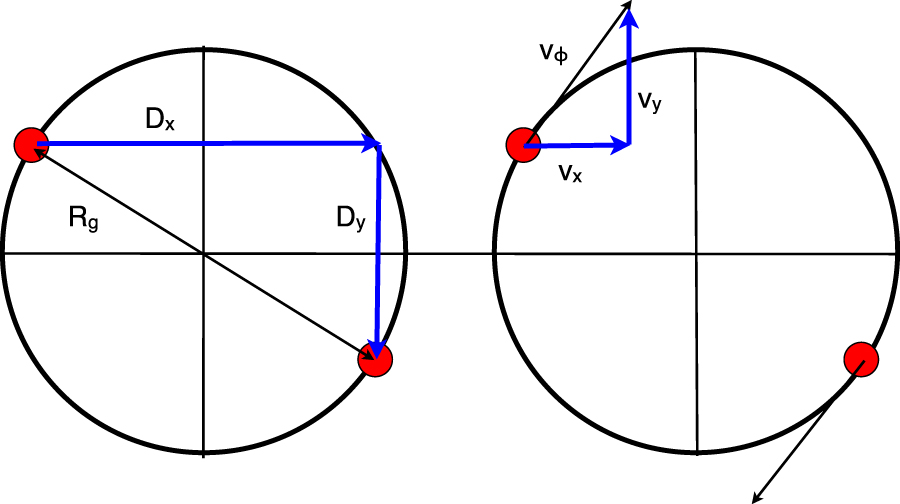
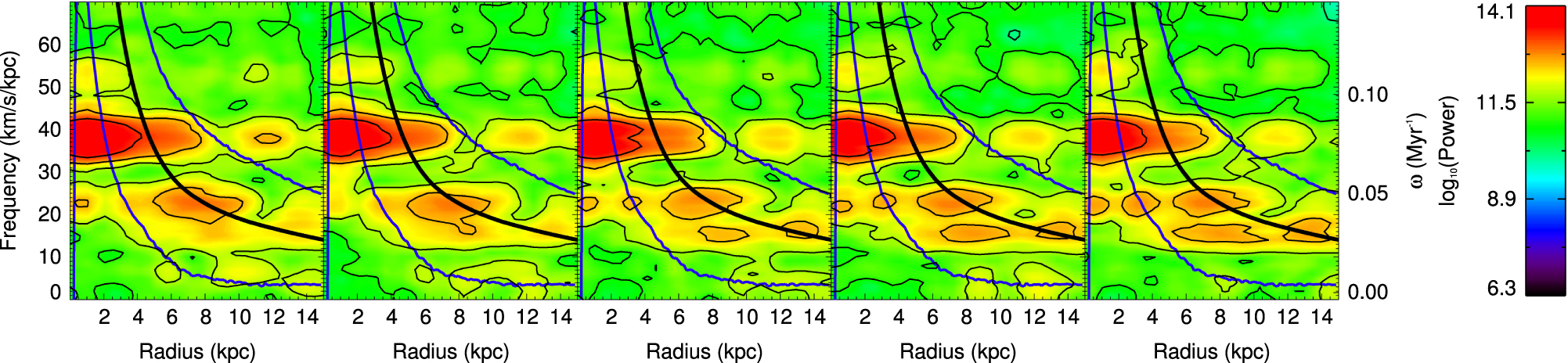
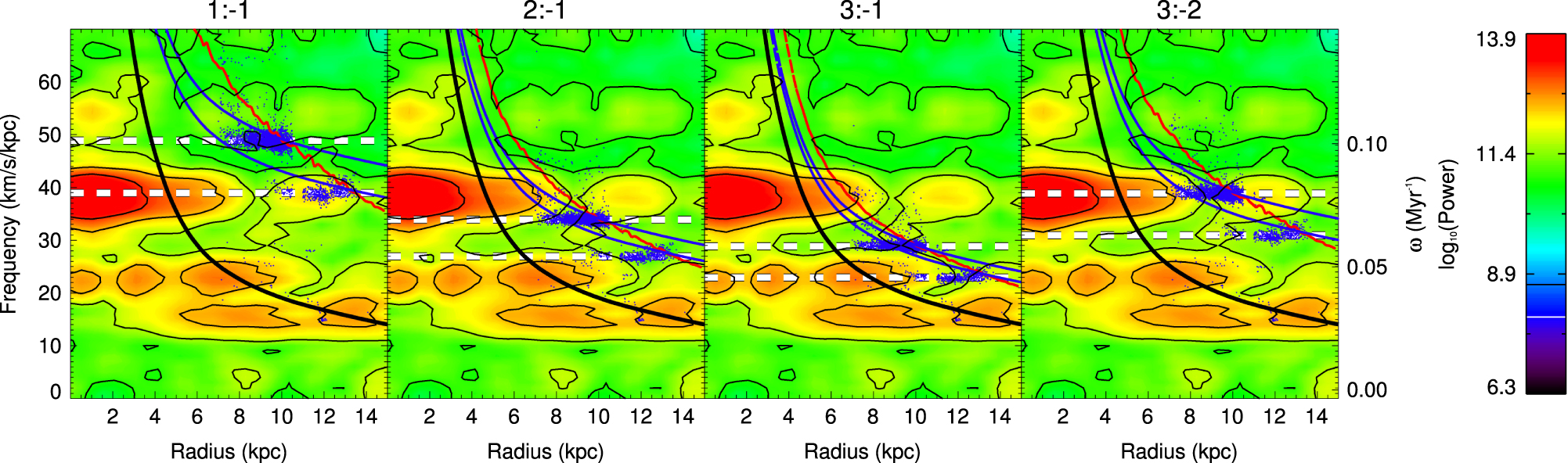
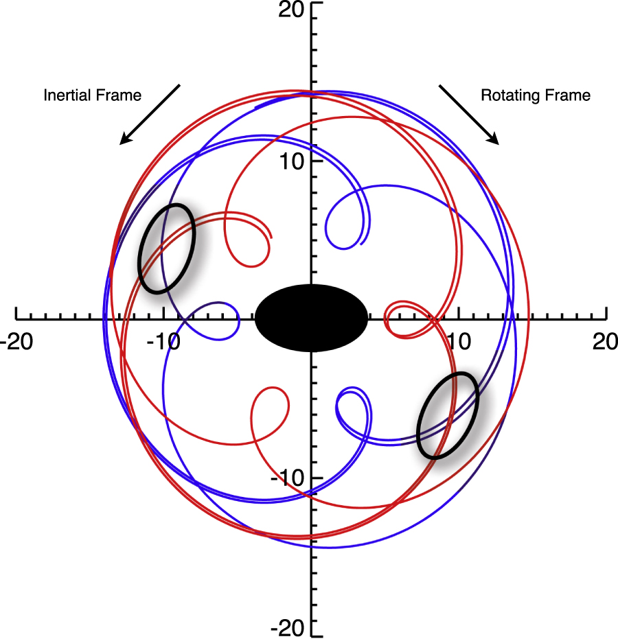
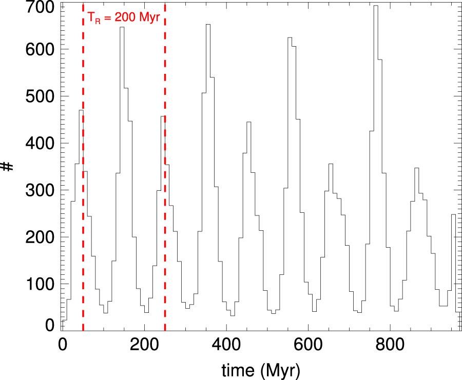
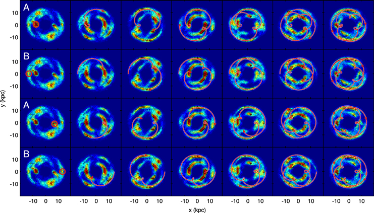
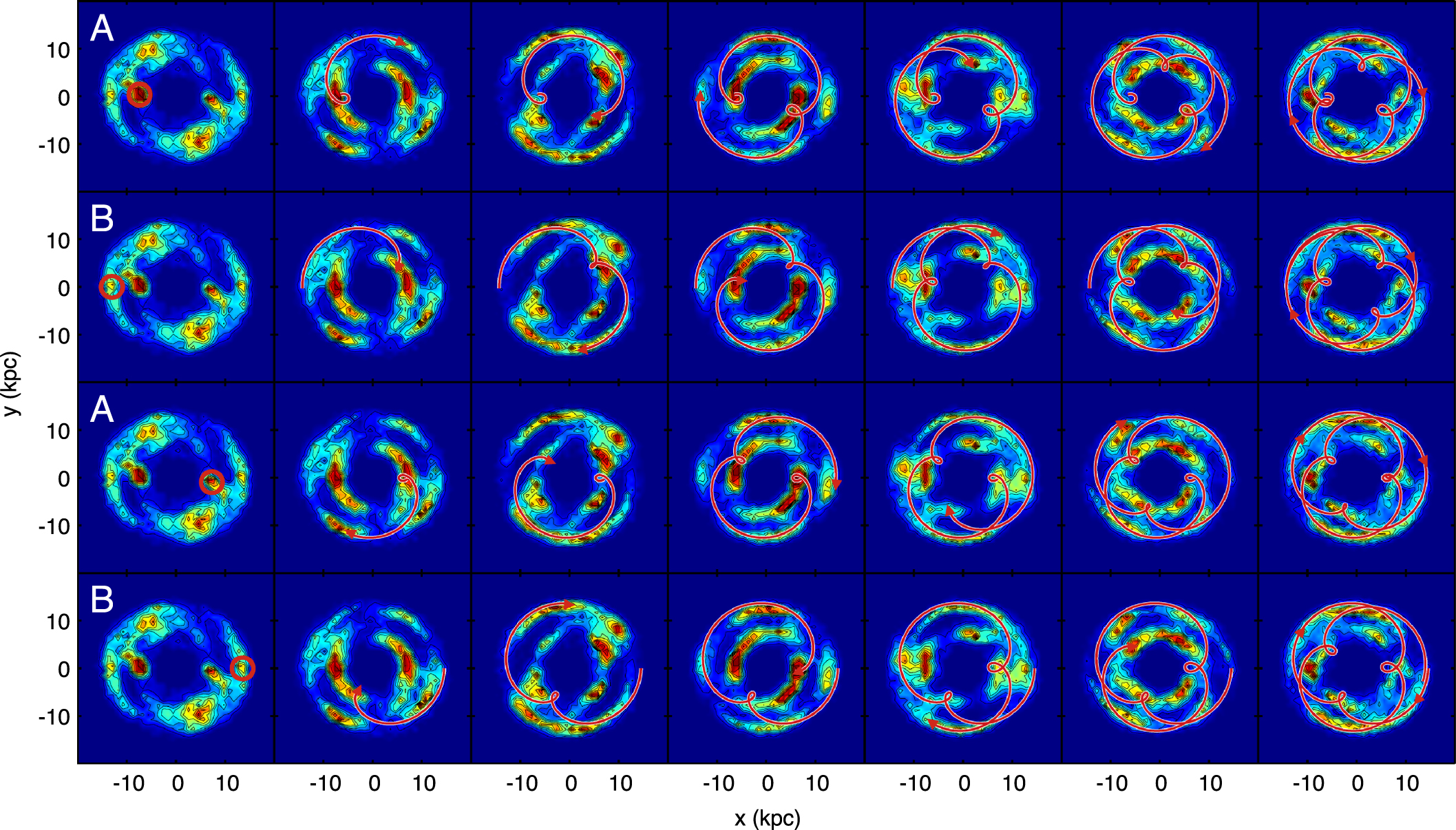
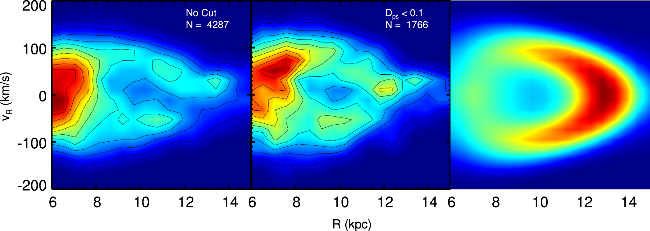
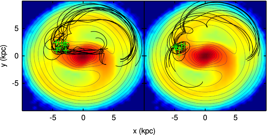
Figure 11. Phase mixing is inefficient, as the clumping in the phase angle  persists for long periods. The pericenter times are shown for the resonant particles common to segments two and eight (highlighted with red on the horizontal axis). The overall distribution of fast actions (
 second row) remains unchanged over the ∼4 Gyr shown here. Individual particles do, however, experience changes in their respective actions shown by the distribution of
  in the third panel. Changes in the fast action are accompanied by changes in the corresponding frequency κ (where
  ).
).
Download figure:
Standard image High-resolution image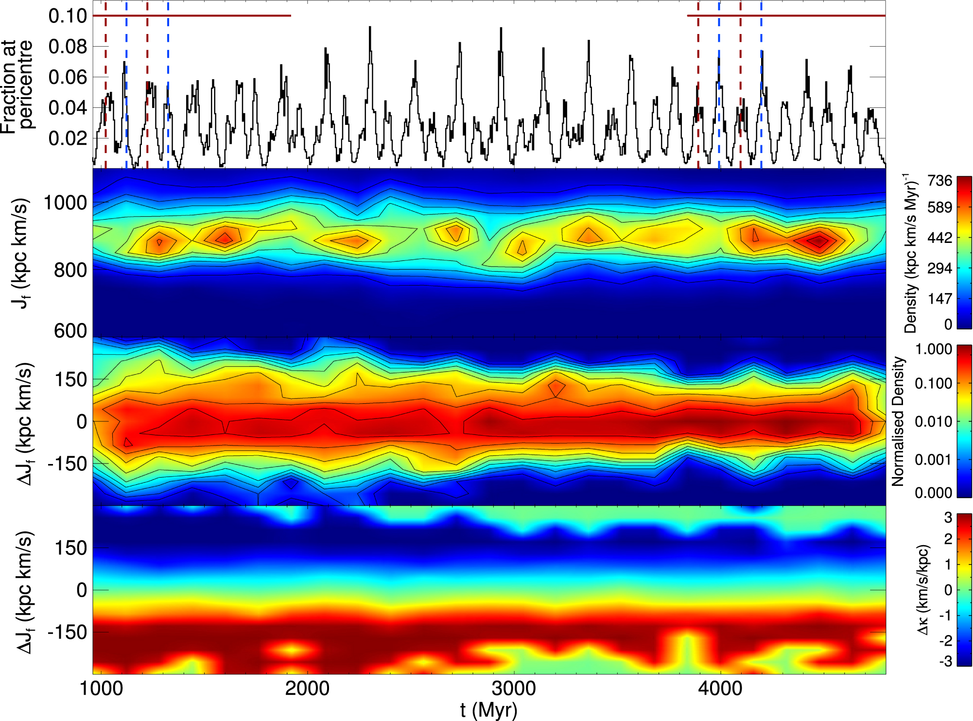
Since the phenomenon of resonant clumping necessarily involves transient overdensities, we suggest that changes in the actions JR and  are working against phase mixing and keeping them locked in phase angle. Below we set out how we measure the actions. Note we do this only for the particles caught in segments two and eight that are deemed to be in a 3:-2 resonance—i.e., those from the top panel of Figure 11.
We compute the actions (J) by numerically integrating over the N-body trajectories. We measure the radial action JR as
where we have integrated over half of the epicycle. The next measurement is taken over the second half of the epicycle. To follow the evolution of the actions, we assign a time to each measurement. If we begin the measurement at  and end it at
  with the duration
  , then we say that orbit has an action JR at time
  . It is also convenient to measure the epicyclic frequency κ as

We measure the azimuthal action as
where  and
and  are the azimuths at which pericenter or apocenter is reached, i.e., the azimuths at
  and
and  from above. In a similar way to our measurement of κ, we reckon Ω as
The fast action  is just a linear combination of JR and
  (see Collett et al. 1997, for details), so that

where m and l are the usual integers describing the closed orbit.  describes the motions of particles along the orbit pattern, whereas the slow action,
  , describes the precession of the apsides of the orbit pattern (the 3:-2 pattern).
Figure 11 (second panel) shows the evolution of the fast actions for the sample of resonant particles extracted from time segments two and eight. The combination of slightly increasing radial actions and slightly decreasing azimuthal actions (not shown) leads to a distribution of fast actions that barely changes. We have also made an estimate of  and
and  , by taking one measurement of
  or κ subtracted from the next. We remark that this is not the time derivative of
  but the change per half epicycle and gives us an idea of the trends in the actions and frequencies. Figure 11 (third panel) shows that although the overall distribution of
  does remain largely constant, there are changes in the actions of individual particles. The changes are most pronounced at earlier times but persist until the later stages of the disk’s evolution. Figure 11 (fourth panel) then shows that the changes in
  (
( ) are accompanied by changes in κ (
 ). This is exactly the same as Figure 11 (third panel), except instead of color representing density, it now represents the average change in κ—blue represents a decrease in κ, and red represents an increase. If, for a particular particle, the fast action has increased, then this is accompanied by a decrease in the corresponding frequency—which is κ in this case. The opposite occurs for a decrease in
  . The distributions of pericenter times show that mixing in the phase angle is not occurring, so that the changes in the frequency κ work against the phase mixing.
6. SUMMARY AND CONCLUSIONS
With the emergence of N-body simulations as the workhorse in the study of galaxy dynamics and evolution, it is important to have the tools available to extract as much information as possible from them. The potential in galaxy disks is inherently time-dependent, driven by evolving bars, rings, and spiral patterns. This then prevents a steady state description of the disk using a time-independent Hamiltonian. Frequency analyses also encounter issues in highly dynamic, unsteady, and evolving systems. When low-frequency orbits occur in varying potentials, it can be hard to separate them from induced radial modes (e.g., Ceverino & Klypin 2007). In disks with significant angular momentum exchange, it can also be difficult to measure the characteristic frequencies of the orbits (κ and Ω).
Resonant orbits play a special role in such systems. We have developed a method to make rapid and automated searches for closed orbits in N-body simulations. This algorithm utilizes the fact that orbits resonating with a bar or spiral pattern in a rotating frame return periodically to a previously inhabited spot in phase space. By defining a metric that measures distance traveled in phase space, we have extracted samples of closed orbits from the simulation of Shen et al. (2010). The sample can be tuned by use of an arbitrary phase-space distance cutoff point. The choice of cutoff depends on how “clean” a sample of closed orbits is required. This essentially separates an N-body simulation into distinct components—the possibly many resonant families and the background disk population. The method has its greatest utility in complex dynamical systems, such as a Galactic bar, where perturbation theory and frequency analysis may have difficulty (see, e.g., M. Molloy et al. 2015, in preparation).
As a worked application, we use the method to dissect the N-body simulation of Shen et al. (2010). This starts as an unstable disk that rapidly forms a massive bar, which evolves through buckling instabilities to give a bulge that is an excellent match to the data in the central parts of the Milky Way. However, a drawback to the simulation is that the outer disk is kinematically hotter than is the case for the Milky Way, which prevents a direct comparison with data. The size of the bar and the absence of both gas and a live halo mean that angular momentum exchange in the disk is maximized. These two aspects of the simulation mean that perturbation theory and a frequency analysis would rapidly encounter their respective limitations.
In the outer disk, we extracted a sample of resonant orbits. By combining the orbital properties of our sample with Fourier spectrograms, we have demonstrated the source of the resonance as the central bar itself (Figure 4). In this simulation, the major populations of resonant orbits are the 3:-2 and 1:-1 families. By measuring the epochs at which closed orbits reach their turning points, we see that they move in a coordinated fashion. The particles that populate these resonant orbits all conspire to reach their pericenters and apocenters at roughly the same time (Figure 7). This leads to the phenomenon of resonant clumping in the disk. Overdensities are produced each time a pericenter or apocenter is reached. These overdensities can make a significant contribution to the disk potential, and their transient nature prohibits a description of the disk by means of a time-independent Hamiltonian.
The family of 3:-2 orbits exists in two distinct groups, whose epicycles are out of phase by π. This means that as one group reaches apocenter, the other reaches pericenter. As the particles complete their respective epicyclic motions, they overlap in configuration space, with one group moving inward, and the other moving outward. This characteristic of their collective motion generates a bimodal distribution of galactocentric radial velocities that occurs at distinct angles with respect to the bar. For the family of 3:-2 orbits, this occurs at angles of between 20° and 40°, which is in the range measured for the viewing angle of the Galactic bar. While we refrain from making a direct comparison with the Milky Way due to the hotness of the simulated disk, we have provided a mechanism that may explain the bimodal distribution of vR observed by Liu et al. (2012) toward the anticenter.
Each group can also be divided into subgroups depending on the azimuth at which they reach their pericenter or apocenter. For example, if one subgroup reaches their pericenter on the negative x axis (i.e., at one end of the bar), another subgroup appears on the positive x axis. This means that, as one overdensity is produced, so another is produced on the opposite side of the disk. This maintains a bisymmetric pattern and prevents the disk from becoming lopsided.
The phenomenon of resonant clumping has not received much attention hitherto. For this reason, we have endeavored to uncover how it comes about, and why it persists in the disk. The global morphology in the density distribution of the resonant particles, along with their proximity to the unstable Lagrange points (and their approach and departure), suggests there is a strong link between the initial clumping mechanism and that which brings about bar-induced spirals—namely, passage through the Lagrange points. Unfortunately, we have been unable to conclusively show how the phase angles become clumped because a reliable measure of  along all points of the orbit is unavailable to us. That the clumping occurs during the formation of the bar is, however, beyond doubt. Since it is likely associated with bar-induced spirals, we suggest that clumping may be responsible for the incomplete or partial rings in barred galaxies (the “pseudorings” or
  rings of Buta 1986). It has been shown that these rings can be generated by stars ejected along the unstable manifolds (e.g., Athanassoula 2012). If the rate of ejection from the Lagrange points is not constant (due to, say, clumping in the phase angle), then we expect incomplete rings to form. The clumping maintains itself by counteracting phase mixing. The transient overdensities provide a force that alters the orbit’s actions and corresponding frequencies. Since we have used very little prior information in extracting these resonant orbits (only the choice of normalization), we have preserved the time-dependent transient nature of processes in the disk.
The release of the Gaia (Perryman et al. 2001) and LAMOST (Deng 2014) data sets will herald a dramatic advance in our knowledge of the kinematic landscape, not only in the Solar vicinity but also to the very edges of the disk. For this reason, it is vital that we have at our disposal the tools required to analyze fully the output from increasingly sophisticated N-body simulations. Deviations from axisymmetry and the resulting resonances must be well understood if we are to comprehend how the Milky Way has evolved. Improving our knowledge of the kinematic structures will help us understand better the importance of secular mechanisms at work in the disk. Decomposing N-body disks into their major orbital components gives us the opportunity to begin to build up analytic models of complex systems by superposing many distinct distribution functions. The method presented here for dissecting simulations should serve as a complementary tool to more established techniques and has the potential to fill in the gaps in our knowledge of galaxy evolution that have yet to be illuminated.
We are deeply indebted to Marcel Zemp and Zhao-Yu Li for many helpful discussions and support during this project. We also thank the referee for insightful comments, which greatly improved the paper. The authors acknowledge financial support from the CAS One Hundred Talent Fund and NSFC grants 11173002, 11333003, 11322326, and 11073037. This work was also supported by the following grants: the Gaia Research for European Astronomy Training (GREAT-ITN) Marie Curie network, funded through the European Union Seventh Framework Programme (FP7/2007-2013) under grant Agreement 264895; the Strategic Priority Research Program “The Emergence of Cosmological Structures” of the Chinese Academy of Sciences, grant XDB09000000; and the National Key Basic Research Program of China 2014CB845700. This work made use of the supercomputing facilities at Shanghai Astronomical Observatory.